What is it?

• Calculating the statistic of interest on “bootstrap resamples” of data
  • Resamples come by sampling with replacement many times
• Seeing Theory

What is the point?

• Estimate statistics when assumptions of parametric models may not hold
• Reduce distortions caused by small sample size

What’s the catch?

• Has its own assumptions:
  • Sample is representative of population
  • Samples are independent

Basic function

library(boot)

boot(data = data,
     statistic = fun, # What function are we using to generate a statistic?
     R=reps # How many times should we repeat this?,
     ... # Can also pass additional parameters to the function
     )

Estimating the mean

# Setup
library(boot)
library(tidyverse)

get_mpg_mean <- function(data, indices){
  # Function has to take in data and indices
  new_data = data[indices,] # Resample based on indices
  return(mean(new_data$mpg)) # Return statistic of interest
}  

# Create the boot object
boot_obj = boot(data = mtcars,
     statistic = get_mpg_mean,
     R = 1000)

boot_obj
## 
## ORDINARY NONPARAMETRIC BOOTSTRAP
## 
## 
## Call:
## boot(data = mtcars, statistic = get_mpg_mean, R = 1000)
## 
## 
## Bootstrap Statistics :
##     original     bias    std. error
## t1* 20.09062 0.06126875    1.049063

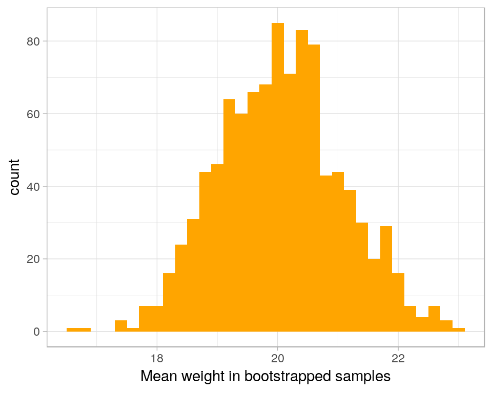
Estimating the mean - visualization

boot_obj$t %>% as.tibble %>% 
  ggplot() +
  geom_histogram(aes(x=V1), fill = 'orange',binwidth=.2) +
  xlab('Mean weight in bootstrapped samples') + 
  theme_light()

Advanced example - bootstrapped confidence intervals for regression

• This should be easier!

get_coefs <- function(data, indices){
  new_data = data[indices,]
  fit_obj = lm(mpg ~ wt + hp + disp, data = new_data) 
  return(coef(fit_obj))
  }
  
boot_obj = boot(data = mtcars,
                statistic = get_coefs,
                R = 2000)

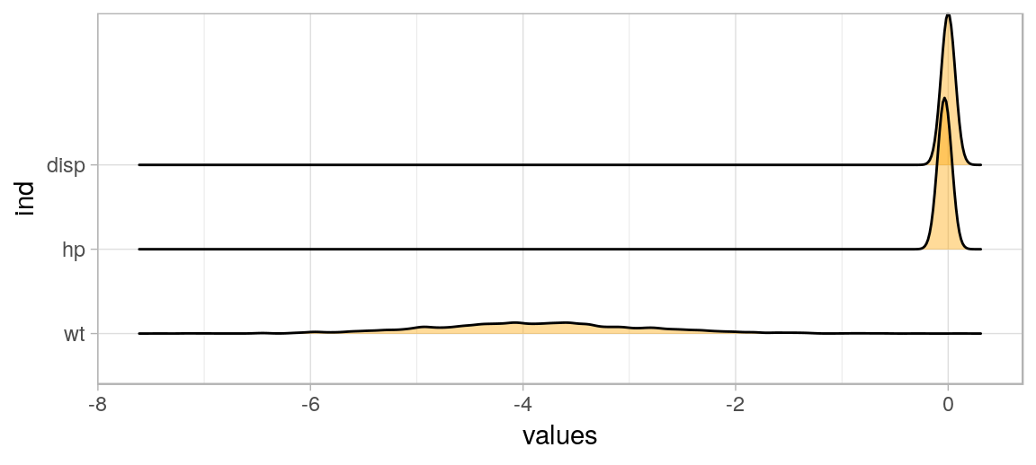
Visualize bootstrapped coefficients

boot_df <- as.data.frame(boot_obj$t)

var_names = names(boot_obj$t0)
colnames(boot_df) <- var_names

library(ggridges)

boot_df %>% stack %>% 
  filter(ind != '(Intercept)') %>%
  ggplot() + theme_light() +
  geom_density_ridges(aes(x=values, y=ind), fill='orange', alpha=.4)

Calculate confidence intervals

simple_cis <- sapply(boot_df, quantile, probs=c(.025, .975))

print(simple_cis)

##       (Intercept)        wt          hp        disp
## 2.5%     32.33534 -5.861030 -0.06023895 -0.01733316
## 97.5%    42.02881 -1.857575 -0.01681910  0.01675699

cis <- sapply(1:length(var_names), 
          function(x) boot.ci(boot_obj, 
                              index=x,
                              type = 'bca')$bca[4:5])

colnames(cis) <- var_names

print(cis)

##      (Intercept)        wt          hp        disp
## [1,]    31.95369 -5.576118 -0.05609859 -0.02235941
## [2,]    41.76300 -1.521268 -0.01415651  0.01381162

Use bootstrapped confidence intervals

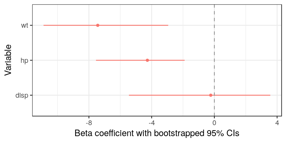
library(dotwhisker)
library(broom)

tidy(lm(mpg ~ wt + hp + disp, data=mtcars), conf.int = T) %>%
  mutate(conf.low = as.numeric(cis[1,]),
         conf.high = as.numeric(cis[2,])) %>%
  by_2sd(mtcars) %>%
  dwplot(show_intercept = F) + theme_bw() +
  theme(legend.position="none") + 
    xlab('Beta coefficient with bootstrapped 95% CIs') + ylab('Variable') + 
    geom_vline(xintercept = 0, colour = "grey60", linetype = 2) #